Quantum tunnelling
| Quantum mechanics | ||||||||||||||||
 |
||||||||||||||||
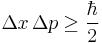
| Uncertainty principle |
||||||||||||||||
Introduction · Mathematical formulations
|
||||||||||||||||
Quantum tunnelling refers to the quantum mechanical phenomenon where a particle tunnels through a barrier that it classically could not surmount because its kinetic energy is lower than the potential energy of the barrier. This tunnelling plays an essential role in several physical phenomena, including radioactive decay and has important applications to modern devices such as the tunneling diode and the scanning tunnelling microscope.[1] The prediction of quantum tunnelling goes back to the very beginning of the 20th century, while its acceptance as a general, physical phenomena would come in the middle of the century.[2]
Quantum Mechanics predicts that a particle has a finite probability of appearing on the other side of any physical barrier, regardless of its height or width. These barriers are any potential energy greater than the kinetic energy of the particle. Quantum tunnelling is a consequence of the wave-particle duality of matter and is often explained using the Heisenberg uncertainty principle. Because purely quantum mechanical concepts are central to the phenomenon, quantum tunnelling serves as one of the defining features of both Quantum Mechanics and the particle-wave duality of matter. And, because of its quantum mechanical nature, the experimental observations of tunnelling provide strong evidence for quantum mechanical theory itself. For this reason, among others, quantum tunnelling is one of the most studied phenomena in the field. Other names for this effect are Wave-mechanical tunnelling, Quantum-mechanical tunnelling, and the Tunnel effect.
Quantum tunnelling is mathematically equivalent to the evanescent wave coupling effect that occurs in optics.
Contents |
History
The theory of quantum tunnelling was born out of the discovery and study of natural radioactivity in the end of the 19th century.[3] This was discovered in 1886 Henri Becquerel.[4] The process was examined further by Marie and Pierre Curie, for which the two shared the Nobel prize in physics.[5] Around this same time Rutherford and Schweidler studied the nature of the decay, later to be verified empirically by Kohrausch. Especially important in their work were the idea of the half life, and that it can only be predicted statistically.[3]
The first to notice the possibility of the mathematical prediction was Friedrich Hund in 1927 when he was calculating the ground state of the double-well potential.[6] However, it received its first real attention as a theory as the mathematical explanation of the alpha decay of atomic nuclei. This was would not come until 1928 by George Gamow and, independently, by Ronald Gurney and Edward Condon.[7][8][9] The two parties simultaneously solved the Schrödinger equation for a model nuclear potential and derived a relationship between the half-life of the particle and the energy of emission that depended directly on the mathematical probability of tunnelling. The success of that theory is one of the greatest feats of quantum mechanics itself.
After attending a seminar by Gamow, Max Born recognized the generality of quantum-mechanical tunnelling. He realized that the tunnelling phenomenon was not restricted to nuclear physics, but was a general result of quantum mechanics that applies to many different systems.[10] Shortly thereafter, both groups considered the case of particles tunnelling into the nucleus. In the years to come tunnelling would receive great attention with the study of semiconductors and the discovery of transistor and diodes, leading to the conclusive acceptance of electron tunnelling in solids by 1957. The work of Giaver and later Josephson would lead to the our understanding of superconductors, especially the BCS theory of superconductivity, and the prediction of supercurrents.[11] Since then the theory of tunnelling has even been applied to the early cosmology of the universe.[12] And, only in the last decade of the 21st century was the tunnelling of an individual atom on a metal surface observed.[13]
Introduction to the Concept
One way to convey the idea of quantum tunnelling is by the use of a simply analogy. For this analogy, quantum particles, such as electrons, photons, atoms, etc. are thought of as climbers and potential barriers are mountains they want to cross. In this situation, the climbers may be able to cross through a mountain that they lack the energy to climb over.[6] Where as other climbers, classical particles, have no choice but to climb over. Though the barrier is impenetrable for classical particles, the quantum particles are said to tunnel through it.
The potential mountain image comes especially from Classical Mechanics where a particle has a position and velocity that can be known exactly at every single time. In this case, one can visualize the particle travelling "up" the potential mountain, that is, farther into the field of whatever force is slowing it down. Since the particle is assumed to have less energy than it takes to surmount the large barrier, it travels back, gaining speed all the way. For instance, the particles in the nucleus are held together by the nuclear force. Each one of those particles lives in a nuclear potential whose position-versus-energy graph has two such mountain potentials, one on each side, that slow the particle down and send it back whenever it tries to cross, making it go back and forth. Of course our classical analogy cannot be enough. Our analogy, and perhaps our intuition, breaks down when we find that the particles can be found on the other side of these barrier. In fact, Quantum Mechanics predicts that they any particle can cross any barrier, it simply has a smaller probability for larger barriers.
The image of a particle literally tunnelling fits quite well in the sense that the particle moves through the barrier since quantum mechanics predicts a finite probability of finding the a particle inside the barrier. In fact, the tunnelling barrier need not have another side to come out on. The particle can simply tunnel in and back out of an infinitely wide barrier, often referred to as barrier penetration. More generally, a particle can be found at any position, even if its energy is less than it would classically have to give up to be there. While this is in contradiction to Classical Mechanics, the justification in Quantum Mechanics comes from the theory's wave-mechanical treatment of matter. That is, it considers that particles have properties that resemble both points and waves, known as the particle-wave duality of matter.
Like most wave-mechanical phenomena, our intuition and physical analogies about quantum tunnelling eventually break down. However, we do have ways to interpret what is going on. One such way involving the Heisenberg uncertainty principle is central to our conceptual understanding of Quantum Mechanics. It defines a theoretical limit on how precisely we can know both the position and the momentum or the energy and time of a particle.[14] This idea is often used to explain the phenomena of tunnelling. The uncertainty principle predicts that for a small amount of time the particle might 'borrow' energy from the system so that it can 'jump' over a mountain.[15] That is, it might have a higher energy than we would expect it to since there is a limit on how precisely we can theoretically know the particle's energy.

The Tunnelling Problem
The following is a qualitative discussion of the quantitative analysis behind quantum tunnelling theory and the concepts and terms that that are used to describe it.
The wave function of a particle summarizes everything that we can know about a physical system.[16] It is for this reason that problems in quantum mechanics center around the analysis of the wave function for a system. Using some mathematical formulation of quantum mechanics, such as the Schrödinger equation the wave function, and ultimately the probability density can be solved for. Specifically, it is found in the limit of large barriers that this probability of tunnelling decreases for taller barriers and decays exponentially with the barrier width.
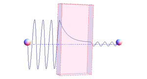
In the figure we see the wave packet of an electron approaching a barrier. The electron's 2-D wave packet represents its localized probability density evolving with time. Brighter spots are represent positions in which the particle is more likely to be found. That is, where the wave packet is most likely localized. The wave packet can be viewed as an ensemble of possible incoming point particles, or a "wave-train". The size of this wave-train depends on the momentum of the particle by means of the Heisenberg uncertainty principle. In many cases, unless the momentum is very large, the scale of the wave-train is as large or larger than the barrier.
For simple tunnelling-barrier models, such as the rectangular barrier, the Schrödinger equation can be solved exactly to give the value of the tunnelling probability (sometimes called the "transmission coefficient"). It is calculations of this kind that have lead to the our understanding of the general physical nature of tunnelling. However, like much of Quantum Mechanics the physically realizeable problems are often beyond exact calculation. Mathematicians and mathematical physicists have been working on problems like this since at least 1813, and have been able to develop special methods for solving equations of this kind approximately yielding lots of excellent results. Many of these approximation are known as "semiclassical" or "quasiclassical" methods. A common semiclassical method is the so-called WKB approximation (also known as the "JWKB approximation"). An outline of one particular semiclassical method is given below.
Related phenomena
There are several phenomena that have the same wave-mechanical behavior. In fact, the same mathematics used in to describe quantum tunnelling, especially the mathematics of the Schrödinger equation, can be used to accurately describe these phenomena. Some examples are the wave coupling effects, which are the application of Maxwell's wave-equation to light, and the application of the non-dispersive wave-equation from acoustics, that is often applied to "waves on strings". Until recently, it has only been in quantum mechanics that evanescent wave coupling has been called "tunnelling". However, there is an increasing tendency to use the label "tunnelling" in other contexts as well, and the names "photon tunnelling" and "acoustic tunnelling" are now used in the research literature.
These effects are often modeled by something similar to the rectangular potential barrier. In these cases, there is one general medium through which the wave propogates that is either the same, or nearly the same throughout, and a second medium through which the wave travels differently. This can be described as a thin region of "medium type 2" being sandwiched between two regions of "medium type 1". To have follow mechanics that are similar to that of the Schrödinger equation applied to the rectangular barrier the properties of these media have to be such that the wave equation has "traveling-wave" solutions in medium type 1, but "real exponential solutions" (rising and falling) in medium type 2.
In optics, medium type 1 might be glass, medium type 2 might be a vacuum. In acoustics, the medium type 2 might be a solid, while the medium type 1 may be a liquid or a gas. Or, it might simply be two strings of different mass-density in the direction of the string. In quantum mechanics, in connection with motion of a particle, medium type 1 is a region of space where the particle's total energy is greater than its potential energy, medium type 2 is a region of space (known as the "barrier") where the particle's total energy is less than its potential energy. All of these wave phenomena will have an incoming wave and resultant waves that both continue on and are refelected back. Of course, like quantum tunnelling, there can be many more mediums and barriers, and the barriers need not be so discrete. However, the simplest approximations are often very useful.
Applications
Tunnelling occurs with barriers of thickness around 1-3 nm and smaller.[17] Nonetheless, it is the cause of some very important macroscopic physical phenemena. For instance, tunnelling is a source of major current leakage in very-large-scale integration (VLSI) electronics and results in the substantial power drain and heating effects that plague high-speed and mobile technology. In fact, it is often considered the lower limit on how small computer chips can be made.[18] Tunnelling has applications in modern physical cosmology, e.g. it runs the fusion reactions that burn in most stars. The following is a list of some of the devices, processes, and theories in which quantum tunnelling plays an essential role.
Radioactive Decay
Radioactive decay is the process by which atomic nuclei release energy by emitting particles, also known as radiation. This is done via the tunnelling of either a particle of particles out of the nucleus, or, in the case of electron capture an electron tunnelling into the nucleus. This phenomena was the first appliction of quantum tunnelling and lead to some of the first approximations used widely in the field. The most prominent breakthrough was the explanation of alpha decay using tunnelling.
Cold Emission
One such application is the cold emission of electrons which is relevant to semiconductors and superconductor physics. It is similar to thermionic emission, where electrons randomly jump off of the surface of a metal to follow a voltage bias because they statistically end up with more energy than the barrier through random collisions with other particles. However, if the electric field is very large the barrier may become thin enough for electrons to tunnel out of its atomic state, leading to a current that varies approximately exponentially with the electric field.[19] These materials are important for Flash memory, a modern form of convenient read/write memory and for some electron microscopes.
Tunnel Junction
One can create a simple barrier for tunnelling by separating two conductors with a very thin insulator (around 1-3 nm). These are called tunnel junctions, the study of which naturally requires quantum tunnelling.[20] Further, Josephson junctions take advantage of quantum tunnelling and the superconductivity of some semiconductors to create an alternating current, known as the Josephson effect. This has applications in extremely accurate measurements that include voltages and extremely small magnetic fields.[21] Also, the tunnel junction has applications to the extremely efficient multijunction solar cell.
Tunnel Diode
Diodes are electrical semiconductor devices that generally allow far greater current in one direction than the other. It uses a semiconductor's large band gap to send electrons in one direction that is favored because the electrons conduct at a higher energy level in the first material than they end in the second. When the voltage is reversed, the electrons have to jump to a higher energy level since it moves from a lower conduction band to a substantially higher one so that there is far less current. When the two semiconductors (called p-type and n-type semiconductors) are very heavily doped the depletion layer can be thin enough for tunnelling. Then, when a small forward bias is applied the current due to tunnelling, or tunnelling current, can be appreciable over the diode. This tunnelling current will have a maximum around the point where the voltage bias is such that the energy level of the p and n conduction bands are the same. However, as the voltage bias is increased the two conduction bands no longer line up and the tunnelling current becomes negligible. At this point the diode acts again as a normal diode.[22]
Because the tunnelling current drops off so rapidly, tunnel diodes can be created that have an range of voltages for which current decreases as voltage is increased. This peculiar property is used in some applications. Also, tunnel diodes are used in high speed devices because the characteristic tunnelling probability changes as rapidly as the bias voltage (without a delay).[23]
The resonant tunnelling diode makes use of quantum tunnelling in a very different manner to achieve a similar result. This diode can have a resonant voltage (for which there is a lot of current) that is much more appreciable than the tunnel diode in both voltage and current, and is used especially to favor a particular voltage. This is done by placing two very thin layers with a high energy conductance band very near each other. This creates a quantum potential well that has a discrete lowest energy level. When this energy level is higher than that of the electrons, no tunnelling will occurs, similar to a diode in reverse bias. However, once the voltage is such that the two energies align, the electrons can flow like and open wire. And, as the voltage is increased further tunnelling becomes improbable again and the diode will likely act like a normal diode again before a second energy level becomes noticeable[24]
Tunnel Injection
Quantum tunnelling composite
Quantum Conductivity
While the Drude model of electrical conductivity made some excellent predictions about the nature of electrons conducting in metals, the model can be furthered by using the theory of quantum tunnelling to explain the nature of the electron's collisions.[25] When a free electron wave packet encounters a long array of uniformly spaced barriers the reflected part of the wave packet interferes uniformly with the transitted one between all the barriers so that the there can be cases of 100% transmission. The theory predicts that if positively charged nuclei form a perfectly rectangular array, electrons will tunnel through the metal like they are free electrons, leading to the extremely high conductance that is observed in these metals. Further the theory predicts that impurities in the metal will disrupt this conductance noticeably.[26]
Scanning Tunneling Microscope
The scanning tunneling microscope, or STM, invented by Gerd Binnig and Heinrich Rohrer, first allowed one to routinely image indicidual atons on the surface of a metal.[27] In 1981 this was a giant leap from the extremely specialized devices that had achieved atomic resolution on a few specific materials. The STM takes advantage of quantum tunnelling probability's extremely sensitive relationship with distance (approximately exponential). This way, when the tip of STM's needle is brought very close to a conductiong surface that has a voltage bias, one can tell extremely sensitively how close the needle is by measuring the current of electrons that are tunnelling across between the needle and the surface. By using piezo rods that change slightly in size when voltage is applied over them the height of the tip can be continuously adjusted to keep the tunnelling current constant. Then, the time-varying voltages that were applied to the piezo rods can be recorded and used to image the surface of the conductor.[28] Today's STM's are accurate to 0.001 nm, or about 1% of an atomic diameter[29]
Enzymes
It has been shown that quantum tunnelling enhances reaction rates in enzymes. Enzymes use tunnelling to transfer both electrons and nuclei such as hydrogen and deuterium. It has even been shown, in the enzyme glucose oxidase, that oxygen nuclei can tunnel under physiological conditions.[30]
Mathematical discussions of quantum tunnelling
The following subsections are for those with a good working knowledge of differential mathematics, as well as familiarity with the theoretical framework developed in the articles: the Schrödinger equation and the WKB approximation .
Schrödinger equation - tunnelling basics
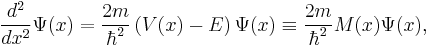
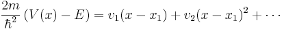
Consider the time-independent Schrödinger equation for one particle, in one dimension. This can be written in the forms

where  is Planck's constant divided by
  is the particle mass, x represents distance measured in the direction of motion of the particle, Ψ(x) is the Schrödinger wave function, V(x) is the potential energy of the particle (measured relative to any convenient reference level), E is that part of the total energy of the particle that is associated with motion in the x-direction (measured relative to the same reference level as V(x)), and
  is a quantity defined by this equation. Explicitly, is given by
 .
.
The quantity has no accepted name in physics generally; the name "motive energy" is used in the article on field electron emission.
The solutions of the Schrödinger equation take different forms for different values of x, depending on whether is positive or negative. This is easiest to understand if we consider a situation in which we have regions of space in which is (a) constant and negative and (b) constant and positive. When is constant and negative, then the Schrödinger equation can be written in the form

The solutions of this equation represent traveling waves, with phase-constant +k or -k. Alternatively, if is constant and positive, then the Schrödinger equation can be written in the form

The solutions of this equation are rising and falling exponentials, which take the form exp(+κx) for rising exponentials, or the form exp(-κx) for decaying exponentials (also called "evanescent waves"). When varies with position, the same difference in behaviour occurs, depending on whether is negative or positive, but the parameters k and κ become functions of position. It follows that the sign of determines the "nature of the medium", with negative M corresponding to the "medium of type 1" discussed above, and positive M corresponding to the "medium of type 2". It thus follows from well-established mathematical principles of classical wave-physics - but applied to the Schrödinger equation - that evanescent wave coupling can occur if a region of positive M is sandwiched between two regions of negative M. This occurs if V(x) has a "hill-type" shape.
A problem is that the mathematics of dealing with the situation where varies with x is intensely difficult, except in certain mathematical special cases that usually do not correspond quantitatively well to physical reality. A discussion of the simple (but quantitatively unrealistic) case of the rectangular potential barrier appears elsewhere. A discussion of the "semi-classical" approximate method, as sometimes found in physics textbooks, is given in the next section. A full (but very complicated) complete mathematical treatment appears in the 1965 monograph by Fröman and Fröman noted below. Their ideas have not yet made it into physics textbooks, but probably in most cases their corrections have little quantitative effect. A brief statement of the outcome of the Fröman and Fröman treatment appears in the article on field electron emission (which was the first major physical effect to be identified as due to electron tunnelling, in 1928), in the section on escape probability.
Note that, in the hypothetical physical picture of "particle" motion used in the 1800s and earlier, in which a "particle" is assumed to have the behaviour of a moving point mass, positive values of correspond to negative values of the kinetic energy of a point mass located at position "x". There is, however, no logical need to introduce the concept of "negative kinetic energy at a point in space" into discussion of evanescent wave coupling (i.e., there is no logical need to introduce this concept into discussions of "tunnelling" based on the Schrödinger equation.)
Applying the WKB method to tunnelling probability
First, express the wave function as the exponential of a function:
 , where
Next, separate the function  into real and imaginary parts:
 , where A(x) and B(x) are real-valued functions.
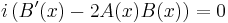
Substituting this new expression back in for and using the fact that the pure imaginary part needs to vanish due to the real-valued right-hand side,
 ,
,
results in:
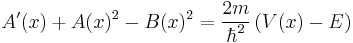 .
.
To solve this equation using the semiclassical approximation, each function must be expanded as a power series in . From the equations it can be seen that the power series must start with at least an order of  to satisfy the real part of the equation. For a good classical limit however, starting with the highest a power of Planck's constant possible is preferable. This leads to:
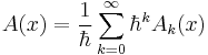
and
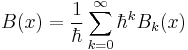 ,
,
with the following constraints on the lowest order terms,

and
 .
.
At this point two extreme cases can be considered:
Case 1
- If the amplitude varies slowly as compared to the phase, we set
 and get
- which is only valid when you have more energy than potential - classical motion. After the same procedure on the next order of the expansion we get
![\Psi(x) \approx C \frac{ e^{i \int dx \sqrt{\frac{2m}{\hbar^2} \left( E - V(x) \right)} + \theta} }{\sqrt[4]{\frac{2m}{\hbar^2} \left( E - V(x) \right)}}](/I/59c905daa195675abf6216e2f08ad32d.png)
Case 2
- If the phase varies slowly as compared to the amplitude, we set
 and get
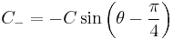
- which is only valid when you have more potential than energy - tunnelling motion. Resolving the next order of the expansion yields
![\Psi(x) \approx \frac{ C_{+} e^{+\int dx \sqrt{\frac{2m}{\hbar^2} \left( V(x) - E \right)}} + C_{-} e^{-\int dx \sqrt{\frac{2m}{\hbar^2} \left( V(x) - E \right)}}}{\sqrt[4]{\frac{2m}{\hbar^2} \left( V(x) - E \right)}}](/I/a8181fce7cb1887dc8c0c2cbb0cfd776.png)
In both cases, it is apparent from the denominator, that both these approximate solutions are bad near the classical turning points,  . The approximate solutions found are for far away from the potential hill, case 1, and beneath the potential hill, case 2. Away from the potential hill, the particle acts similarly to a free wave - the phase is oscillating. Beneath the potential hill, the particle undergoes exponential changes in amplitude.
Now that the behavior at the limits is known an effort can be made to make approximate solutions everywhere and match coefficients to make a global approximate solution. This can be done by considering the classical turning points.
Choose a classical turning point,  . Now expand
  in a power series about giving:
Make a linear approximation by only keeping the first order term,
 .
.
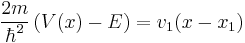
Using this aproximation, the equation near becomes,
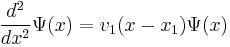 .
.
This differential equation can be solved using Airy functions as its solutions.
![\Psi(x) = C_A Ai\left( \sqrt[3]{v_1} (x - x_1) \right) + C_B Bi\left( \sqrt[3]{v_1} (x - x_1) \right)](/I/4abb5ca637ad527f20ddc4d3a6714beb.png)
Taking these solutions for all classical turning points, a solution can be "chained together" linking the far away and beneath solutions. Given the 2 coefficients on one side of a classical turning point, the 2 coefficients on the other side of a classical turning point can be determined by using this local solution to connect them.
Since, the Airy function solutions will asymptote into sine, cosine and exponential functions in the proper limits. The relationships between  and
and  can be found as follows:
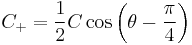
With the coefficients found, the global solution can be solved and tunnelling probabilities found.
The transmission coefficient, 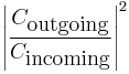 , for a particle tunnelling through a single potential barrier is found to be:
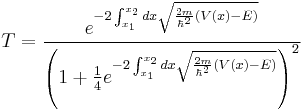 ,
,
where  are the 2 classical turning points for the potential barrier.
To check the validity of this solution, observe that the transmission coefficient correctly goes to zero in the limit  .
.
See also
- Fowler-Nordheim tunnelling
- Dielectric Barrier Discharge
- Holstein-Herring Method
References
- ↑ Taylor, J: Modern Physics, page 234. Prentice Hall, 2004.
- ↑ Mohsen Razavy, "Quantum Theory of Tunneling", page 4. World Scientific Publishing Co. 2003
- ↑ 3.0 3.1 Mohsen Razavy, "Quantum Theory of Tunneling", page 1. World Scientific Publishing Co. 2003
- ↑ Nimtz and Haibel, "Zero Time Space", page 1. WILEY-VCH Verlag GmbH & Co. 2008.
- ↑ Nimtz and Haibel, "Zero Time Space", page 2. WILEY-VCH Verlag GmbH & Co. 2008.
- ↑ 6.0 6.1 Nimtz and Haibel, "Zero Time Space", page 3. WILEY-VCH Verlag GmbH & Co. 2008.
- ↑ R W Gurney and E U Condon, "Quantum Mechanics and Radioactive Disintegration" Nature 122, 439 (1928); Phys. Rev 33, 127 (1929)
- ↑ Interview with Hans Bethe by Charles Weiner and Jagdish Mehra at Cornell University, 27 October 1966 accessed 5 April 2010
- ↑ Friedlander, Gerhart; Kennedy, Joseph E; Miller, Julian Malcolm (1964). Nuclear and Radiochemistry, 2nd edition. New York, London, Sydney: John Wiley & Sons. pp. 225–7. ISBN 978-047-186-2550.
- ↑ Mohsen Razavy, "Quantum Theory of Tunneling", page 3. World Scientific Publishing Co. 2003
- ↑ Mohsen Razavy, "Quantum Theory of Tunneling", page 4-5 World Scientific Publishing Co. 2003
- ↑ A. Vilenkin (2003)
- ↑ Mohsen Razavy, "Quantum Theory of Tunneling", page 5 World Scientific Publishing Co. 2003
- ↑ Nimtz and Haibel, "Zero Time Space", page 5. WILEY-VCH Verlag GmbH & Co. 2008.
- ↑ Mohsen Razavy, "Quantum Theory of Tunneling", page 11. World Scientific Publishing Co. 2003
- ↑ Bjorken and Drell, "Relativistic Quantum Mechanics", page 2. Mcgraw-Hill College, 1965.
- ↑ Lerner and Trigg, "Encyclopedia of Physics 2nd Ed.", pg 1308, VCH Publishers (1991).
- ↑ http://psi.phys.wits.ac.za/teaching/Connell/phys284/2005/lecture-02/lecture_02/node13.html,"Applications of ``tunneling". Simon Connell 2006.
- ↑ Taylor, J: Modern Physics, page 479. Prentice Hall, 2004.
- ↑ Lerner and Trigg, "Encyclopedia of Physics 2nd Ed.", pg 1308-1309. VCH Publishers, 1991.
- ↑ Taylor, J: Modern Physics, page 484. Prentice Hall, 2004.
- ↑ Kenneth Krane, "Modern Physics", pg 423. John Wiley and Sons, 1983.
- ↑ Kenneth Krane, "Modern Physics", pg 424. John Wiley and Sons, 1983.
- ↑ R. D. Knight, "Physics for Scientists and Engineers: With Modern Physics", pg 1311. Pearson Education, 2004.
- ↑ Taylor, J: Modern Physics, page 429. Prentice Hall, 2004.
- ↑ Taylor, J: Modern Physics, page 430. Prentice Hall, 2004.
- ↑ Taylor, J: Modern Physics, page 473. Prentice Hall, 2004.
- ↑ Taylor, J: Modern Physics, page 475. Prentice Hall, 2004.
- ↑ R. D. Knight, "Physics for Scientists and Engineers: With Modern Physics", pg 1310. Pearson Education, 2004.
- ↑ Quantum catalysis in enzymes: beyond the transition state theory paradigm
Further reading
- N. Fröman and P.-O. Fröman (1965). JWKB Approximation: Contributions to the Theory. Amsterdam: North-Holland.
- Razavy, Mohsen (2003). Quantum Theory of tunneling. World Scientific. ISBN 981-238-019-1.
- Griffiths, David J. (2004). Introduction to Quantum Mechanics (2nd ed.). Prentice Hall. ISBN 0-13-805326-X.
- Liboff, Richard L. (2002). Introductory Quantum Mechanics. Addison-Wesley. ISBN 0-8053-8714-5.
- Vilenkin, Alexander; Vilenkin, Alexander; Winitzki, Serge (2003). "Particle creation in a tunneling universe". Physical Review D 68: 023520. doi:10.1103/PhysRevD.68.023520. http://arxiv.org/abs/gr-qc/0210034.